Summarizing data mathematically

Mathematical summarization equips us with the tools to unveil patterns, draw insights, and make informed decisions based on raw datasets. Being able to represent a subset of data using a single vector is a fundamental component of many machine learning algorithms. It is core to our process of drawing any insights from data.

Often, practitioners simply gloss over the choice of summarization techniques, focusing more on the choice of algorithm or the metric. While those are also important things, and I will discuss them at length in other articles, in this article I would like to spend time showcasing the vastness of the topic of summarization. Here are the fundamental ways to summarize data mathematically:

Measures of central tendency

Mean: Most common. Useful for symmetric distributions.
Median: Midpoint separating lower/upper 50%. Robust against outliers.
Mode: Most frequent value. Relevant for categorical/discretized data.

Special case: geometric mean and exponential decay

Assume you have a dataset representing the monthly decay of a radioactive element. This data would likely follow an exponentially decaying distribution, where the value decreases at a constant rate over time.

Plot showing Radioactive Decay

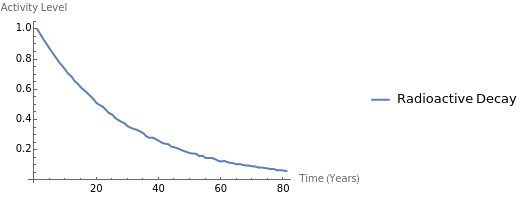
Arithmetic Mean vs. Geometric Mean: The arithmetic mean (average) in this case might be misleading. It would be overly influenced by the higher initial values, not giving an accurate picture of the ongoing decrease. The geometric mean, however, would provide a more realistic idea of the average decay rate over time. This is because it takes the nth root of the product of all the values, essentially capturing the overall multiplicative effect of the decay.

Arithmetic Mean: Ā = ( Σ xi ) / n

Geometric Mean: GM = ⁿ√(x₁ * x₂ * ... * xn)

Harmonic Mean: HM = n / ( Σ (1/xi) )

Σ signifies "sum of"

xi represents each individual data point

n is the total number of data points

ⁿ√ signifies the nth root

Intuition for exponential data: Ā > GM > HM

Different perspectives on the data

While the geometric mean focuses on the overall decay trend, the harmonic mean offers a complementary perspective:

Slow Rates Matter More: The harmonic mean is heavily influenced by very small values. In the context of decay rates, it would be more sensitive to the slow decay rates in the later stages, where the values are much smaller. This can be useful if you're interested in the time it takes for the values to reach a certain threshold or become negligible.

Choosing the right mean

Overall Decay Trend: Geometric mean is a good choice to understand the average rate of decay over time.
Sensitivity to Slow Rates: Harmonic mean is useful if you're more interested in how long it takes for the values to decay significantly.
Symmetrical Distribution: Arithmetic mean remains appropriate for symmetrical distributions without extreme values and strong trends.

Measures of dispersion (spread)

Range: Difference between max/min values. Influenced by extremes.
- Range = Maximum Value - Minimum Value
Interquartile Range (IQR): Spread of middle 50% of data. Less outlier-sensitive.
- IQR = Q3 - Q1
  - Q3 is the third quartile (75th percentile)
  - Q1 is the first quartile (25th percentile)
Variance: Average squared deviation from mean.
- σ² = ( Σ (xi - Ā)² ) / n (or ( Σ (xi - Ā)² ) / (n-1) for population variance)
  - Σ signifies "sum of" for all data points (i = 1 to n)
  - xi represents each data point (value)
  - Ā is the mean
  - n is the total number of data points
Standard Deviation: Square root of variance. Interpretable units.
- σ = √σ²
  - σ² is the variance

Measures of shape

This group of measures are the most interesting when the values themselves are not discriminative but the shape of the distribution over a time window is.

Skewness: Asymmetry of a distribution.
- Positive skew = longer tail on the right
- Negative skew = longer tail on the left
- Zero skew = perfect symetry
Kurtosis: "Peakedness" of distribution.
- High kurtosis = tall, sharp peak
- Low kurtosis = flatter, wider peak

Visual summaries

Beyond numerical measures, visualizations offer powerful ways to summarize data mathematically:

Histograms: Frequency distribution visualization.
Box Plots: Visual median, quartiles, outliers.

Windowing functions and frequencies

Windowing functions are powerful tools for analyzing time-series data in the frequency domain. They , similar to finding modes within discretized frequency ranges.

We saw some measures of shapes above, which are incredibly valuable with windowing functions. Windowing functions are more powerful however as they can capture some patterns in many other ways. One example of this is in the frequency domain.

Discrete Fourier Transform (DFT): Highlight dominant frequencies within specific time windows.
- In a simplified way, this is analogous to finding the "mode" within a discretized range of frequencies.

Embeddings

The curse of high dimensionality

Working with high-dimensional data comes with several challenges:

Computational Complexity: As the number of dimensions (features) grows, many operations become computationally expensive.
Sparse Data: Data points spread out in high-dimensional space become very distant from each other.
Loss of Intuitiveness: Geometric concepts like distances and clusters become less intuitive and can be misleading.

Benefits

Embedding techniques project high-dimensional data onto a lower-dimensional space without loosing as much information as the techniques discussed previously in this article.

Similarity Measures: Calculating similarity measures (e.g., cosine similarity, Euclidean distance) becomes more meaningful. This improves accuracy in clustering and anomaly detection.
Visualization: Projecting data into 2D or 3D with embedding techniques like t-SNE or UMAP allows us to gain visual insights into possible patterns or trends within our complex tabular data.

Beyond central tendencies

While the means in Euclidean space summarize a group of points with a single point, embedding methods are far more flexible:

Non-Linear Relationships: Embeddings can project data onto manifolds, capturing complex, non-linear patterns.
Preserving Information: Good embedding techniques strive to retain information about the original data relationships, even in a lower dimension.
Data-Driven Projections: The embedding process often "learns" the ideal low-dimensional representation from the data itself, making it adaptive and versatile.

Examples of embedding techniques

Principal Component Analysis (PCA): One of the classic dimensionality reduction techniques, PCA finds linear combinations of features that capture the most variance in the data.
t-SNE (t-distributed Stochastic Neighbor Embedding): Popular for visualization, t-SNE preserves the local structure of the high-dimensional data.
Autoencoders: Neural network-based techniques that learn an encoder to compress the data and a decoder to reconstruct it from its lower-dimensional representation.
Word Embeddings (Word2Vec, GloVe): Though originating in natural language processing, these techniques can be adapted for tabular data as well, projecting categorical variables into meaningful vectors.

Important considerations

Choosing the Right Technique: Different embedding methods have different strengths (e.g., linear vs. non-linear, preserving global vs. local structure).
Evaluation: Embedding quality is often assessed using downstream tasks (e.g., performance of clustering algorithms on embedded data). It's important to benchmark against your desired use case.

Conclusion

Choosing the appropriate methods for summarizing data depends heavily on the nature of your data and the questions you're trying to answer. These factors include the data types in the raw or featurized data, the distribution shapes, and presence or absence of outliers. We often see Notebooks were data exploration is done for the sake of it without later using that information for feature construction.

Careful feature construction can help even for problems being solved by deep learning. The same has been discussed in seminal papers by big-tech companies. I will discuss more about these real-world examples in future posts.